May 31, 2023

Quantification of Model Uncertainty (Part 2)

Juan Martinez

Introduction

While Model Risk Management (MRM) principles are important, meeting the expectations set by regulators (FED 2011, PRA 2023) and fostering a robust risk management framework can be challenging or even confusing at times. We believe all MRM practitioners must develop a good understanding of these principles and actively implement them into the organization’s risk management culture.

Embarking on the second journey of our series dedicated to uncertainty in model risk management, it’s important to keep in mind the crucial points we covered in Understanding Uncertainty for Model Risk Management (Part 1). Recognizing the significance of uncertainty in the modelling process and adopting a prudential modelling culture is not only beneficial, but essential in making informed business decisions.

We previously highlighted how a systematic approach to uncertainty can lead to more transparent and accountable models, robust testing during model development, and an effective challenge between the first-line and second-line of defense. Additionally, it enables us to create quantifiable metrics for risk appetite, identify early warning indicators for ongoing monitoring, generate challengeable metrics for model tiering, and implement effective model conservatism.

However, acknowledging and implementing these practices are only the first steps in managing model uncertainty. Given that the ultimate purpose of quantitative models is to present the most plausible options rather than definitive answers, we must understand how model uncertainty arises.

In this second article, we will take a deeper dive into model uncertainty. We’ll explore quantitative methods for assessing uncertainty using simple modelling case studies that will help us gain a more comprehensive understanding of the principles and practices we discussed in part one.

We hope to offer model risk professionals with more tangible, actionable insights around this important topic that can help efficiently navigate the current and new model risk management regulatory demands.

Interpreting Uncertainty

Understanding the different sources of uncertainty is valuable for assessing which deficiencies can potentially be mitigated by further investigation in many cases. This has direct applications in model risk regulation, such as the previously mentioned Margin of Conservatism. Appropriate quantification of uncertainty is also important to communicate model results transparently and avoid creating a false sense of risk to users. When using intervals around point estimates, it is important to know, for example, whether those intervals correspond to random variations around the long-term mean (aleatoric uncertainty) or the actual point estimate (the combination of aleatoric and epistemic uncertainty, defined earlier as model uncertainty). Both can be useful, if they are understood. However, prediction points are indeed more difficult to predict than the expected mean, so the prediction intervals (uncertainty around the point estimate) will be wider than the confidence intervals (uncertainty about the mean).

We illustrate model uncertainty in a classical statistical setting. These examples, although simple, are key building blocks of widely used models in finance. The concepts explained here can be applied to more general cases beyond linear regression, such as Generalised Linear Models, Time Series models or a combination of models.

A Simple Case

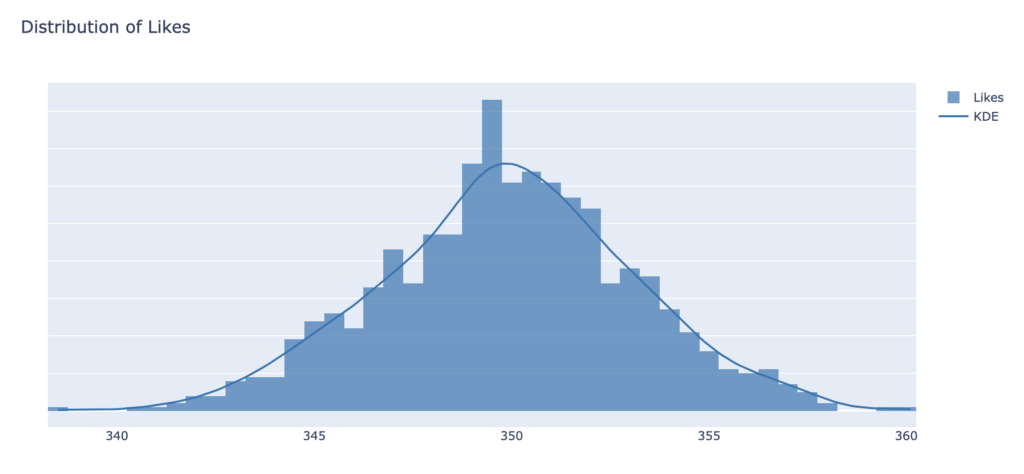
Suppose that one of the inputs to your decision-making model is an estimate of how many like-dislike feedbacks in the next quarter will be likes, knowing that you receive 500 feedbacks per quarter and on average, 70% are likes. The natural thing to do seems obvious, and is to set a fixed parameter:

$LIKES=350$

However, if we see all quantitative estimates as what they really are, wrong by nature (Box, 1976), the average $0.7$ will be perceived not as a fixed parameter, but rather as the most plausible estimate of that parameter. The next question for a prudential modeller then is: how can I extract all the plausible parameter values given the data?

In this simple example, we can represent the data as an independent 1/0 process likes which can be appropriately modelled, although only as an approximation, with a binomial distribution with model parameters $n_{feedbacks}=500$ and $p_{like}=0.7$ :

$likes \sim Binomial(n_{feedbacks},p_{like})$

We can now produce a point estimate for the parameter $LIKES$ . After sampling once from the Binomial distribution $likes$ , we obtain:

$LIKES = 358$

To extract variability around the parameter estimate 0.7 (aleatoric uncertainty), we repeat the same experiment multiple times, by sampling multiple times (1000 is good enough) from the likes distribution:

$LIKES =Binomial(500,0.7,1000)$

The modeller can now use this distribution to, for example, propagate uncertainty to downstream models, or to perform a risk impact assessment against different parameter values and assign probabilities to those scenarios.

Linear Regression

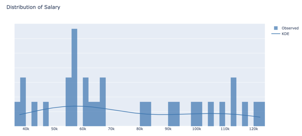
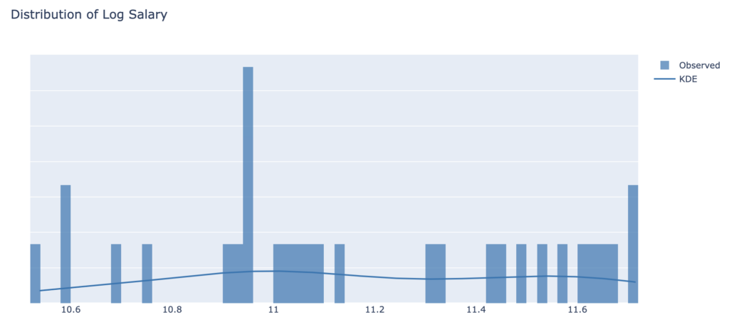
We now build a simple linear regression model to illustrate model uncertainty in a slightly more realistic setting. We try to predict the salary of employees based on their years of experience. We notice that the scale of the target and explanatory variables is significantly different, so we proceed to normalise the dataset by applying the logarithm to the salary. The table below shows the main features of the dataset:

Measure	Years of Experience	Salary	Log Salary
n	30	30	30
min	1.1	37,000	10.5
mean	5.3	76,000	11.17
max	10.5	122,000	11.72

We draw histograms to identify the distribution of our data, that may inform the modelling choices:

We check the relationship between Years of Experience and Log Salary:

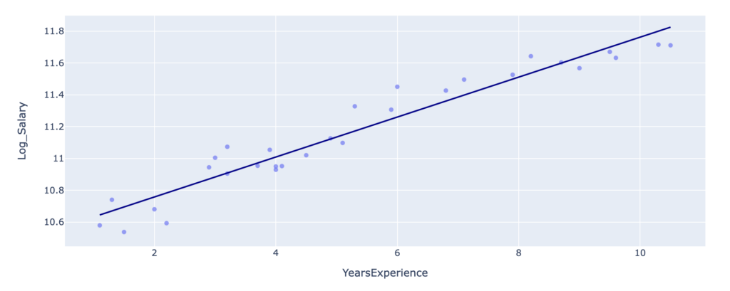
This relationship can be approximated by a classical linear regression model:

$Log(Salary)=\alpha + Experience\cdot \beta + \epsilon$

where $\alpha$ represents the intercept, and $\beta$ the coefficient estimate for the years of experience. In this specification, the error term of the model $\epsilon$ (observed vs predicted) assumes an independent normal distribution with mean 0 and standard deviation $\sigma$ :

$\epsilon =N(0,\sigma^{2})$

After fitting this regression model to the available data, we obtain the following estimates:

$\hat{\alpha}=10.5; \hat{\beta}=0.13; \hat{\sigma}=0.1$

We can now use this specification to produce a point estimate that predicts, for example, the salary of a person with 15 years of experience:

$\hat{Log(Salary)}=10.5+0.13\cdot 15 \pm 0.1= 12.5 \pm 0.1$

We obtain the Salary predictive mean and standard deviation by exponentiating the model output:

$\hat{Salary}=e^{12.5}\pm e^{0.1}\sim 268000 \pm 1.1$

Sources of Model Uncertainty

The epistemic uncertainty in this model (the lack of knowledge about the data generating process) is captured by $\hat{\sigma}$ , the standard deviation of the residuals. In other words, a measure of the average distance of each observation from its model prediction. This error can be potentially reduced by improving the model. The second source, aleatoric uncertainty (variance in the model parameters), is embedded in the estimates $\hat{\alpha}$ and $\hat{\beta}$ .

Defining Uncertainty in the Model

One useful way to visualise these variances is to write the model in probabilistic terms, where each parameter of the model is represented by probabilities distributions $\alpha$ , $\beta$ and $\sigma$ , centred around the model estimates $\hat{\alpha}$ , $\hat{\beta}$ and $\hat{\sigma}$ , respectively:

$\hat{Log(Salary)}=N(\alpha+Experience\cdot\beta, \sigma)$

Where:

$\begin{bmatrix} \alpha \\ \beta \end{bmatrix}= MN\begin{pmatrix} \begin{bmatrix} \hat{\alpha} \\ \hat{\beta} \end{bmatrix},V\cdot \hat{\sigma}^2 \end{pmatrix}$

the multivariate normal distribution $MN$ includes the univariate distributions for $\alpha$ and $\beta$ with mean $\hat{\alpha}$ and $\hat{\beta}$ , respectively, and variance capturing the parameter uncertainty (or epistemic uncertainty), represented by $V\cdot\hat{\sigma}^{2}$ . The latter is the estimated covariance matrix of the model parameters, where $V$ is the unscaled estimated covariance matrix. Note that, usually, the output of model fits gives the scaled version ( $V\cdot\hat{\sigma}^{2}$ ) of the estimated covariance matrix. The diagonal elements in $V\cdot\hat{\sigma}^{2}$ are the estimated variances of $\alpha$ and $\beta$ , and the off-diagonal elements represent the correlation of these predictors.

Next, we extract the aleatoric uncertainty from our model by adding variability to the model error term $\epsilon$ , using a chi-squared distribution (appropriate for modelling variances):

$\epsilon \sim N(0,\sigma^{2})$

Where:

$\sigma=\hat{\sigma}\cdot\sqrt{(n-k)/\chi^{2}}$

with $n$ as the number of data points (30) and $k$ the number of predictors (2).

Extracting Uncertainty from the Model

We can now simulate from this probabilistic model (Gelman, 2007) and extract uncertainty from the previously estimated parameters and the error term:

$\hat{\alpha}=10.5; \hat{\beta}=0.13; \hat{\sigma}=0.1$

For each draw out of the number of simulations (example: 1000):

$\sigma_{i}=\hat{\sigma}\cdot \sqrt{n_{obs}-n_{predictors}}/\chi^{2}(n_{obs}-n_{predictors},1)$

The results of this inferential simulation produce univariate distributions $\alpha$ , $\beta$ and $\sigma$ , for each model estimate $\hat{\alpha}$ , $\hat{\beta}$ and $\hat{\sigma}$ , coherent with this dataset and this model:

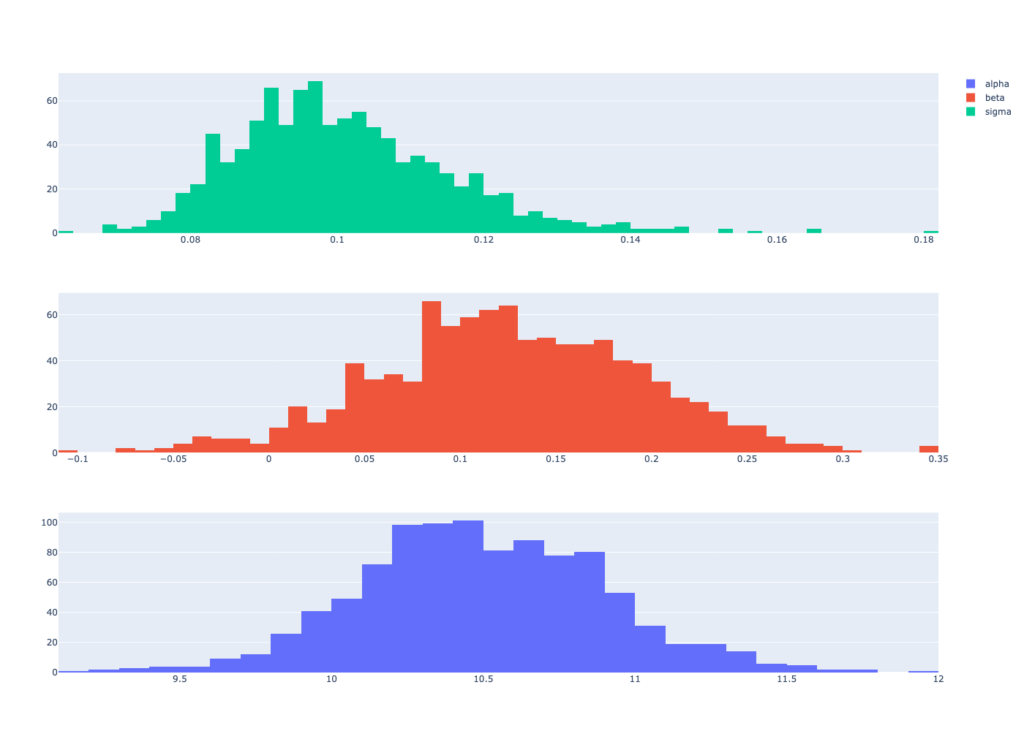
This gives us flexibility in propagating uncertainty about any combination of plausible values of parameters and model errors, based on the data available.

Predictions Accounting for Model Uncertainty

The final step is to obtain predictions using the estimation uncertainty around the coefficient estimates and the error term of the model. To accomplish this, we compute multiple predictive paths following these simple steps:

We generate simulations from the probabilistic model that accounts for uncertainty in both the coefficient estimates and the model error. The simulations are designed to take into account both epistemic and aleatoric uncertainty. The generation of multiple possible paths of outcomes during the simulations reflects these uncertainties and helps capture a range of possible future scenarios.
Once the simulations are completed, the generated data for all the simulated paths are combined into a single dataset. This dataset represents the spectrum of potential outcomes considering the aforementioned uncertainties. This combined dataset forms the basis for the subsequent analysis and visualization of the simulated outcomes.

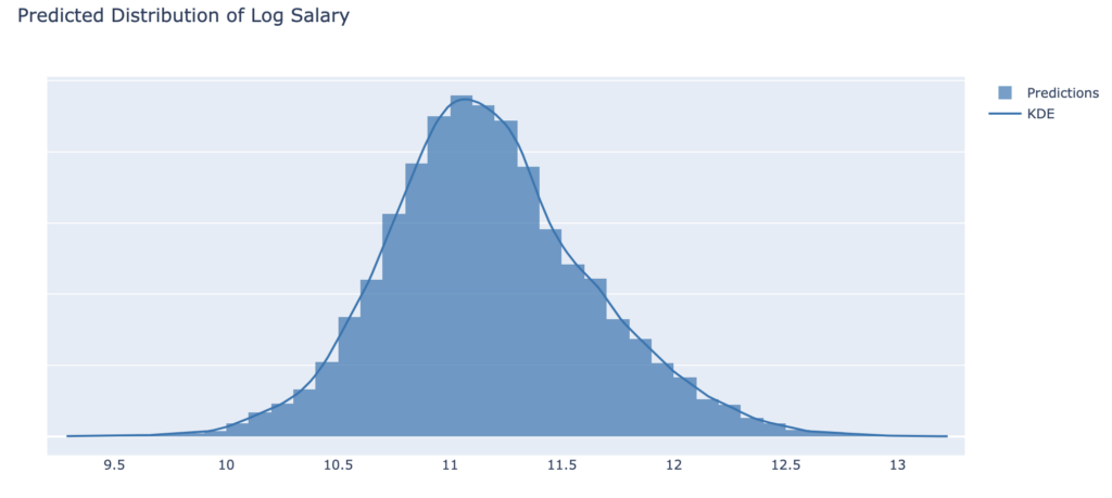
The figure below shows the predictive distribution of Log Salary, created from the above simulation procedure, that captures both sources of model uncertainty:

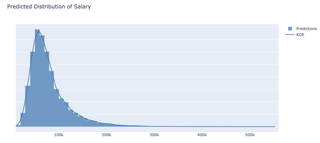
After applying $exp$ , we obtain the Salary levels:

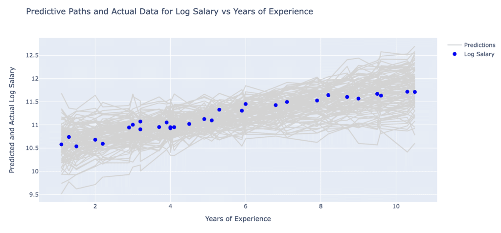
These simulations model potential paths for the relationship between years of experience and log salary, accounting for the model uncertainties involved. For example, a given amount of experience might lead to different salaries depending on other unknown or uncontrolled factors, and this is shown in the forecast plots below, both for Log Salary and Salary.

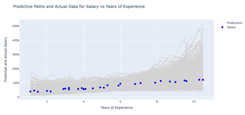
We can see in this plot that salary distributions are often observed to be right-skewed. This may mean, for example, that there are a small number of individuals with very high incomes while the majority of individuals have relatively lower incomes.

These uncertainty measures can serve, for instance, as a basis for setting risk appetite, allowing banks to establish appropriate thresholds for acceptable deviations in salary projections. Moreover, incorporating an add-on derived from the uncertainty analysis, we can prudently account for potential variations in salaries over business planning projections.

The integration of uncertainty into critical models ensures a more realistic and robust approach, enabling financial firms to strategically allocate resources in the face of uncertain assumptions.

Conclusions

In this second part of the series, we presented a validation practice to deconstruct and understand model uncertainty. This involves creating predictions against different scenarios as a combination of different levels of aleatoric and epistemic uncertainty (examples: severe, medium, baseline). We can compute these different prediction paths by sampling different parts of the distribution of the model estimates (epistemic) and standard error (aleatoric).

We can also entirely switch off and on different sources of uncertainty and see the impact on predictions. This can be used to set for example Post Model Adjustments (PMAs) tailored to different model deficiencies, as opposite to use one general PMA to mitigate the overall model error. A more granular approach to PMAs allows MRM professionals to challenge the effectiveness and usage of these PMAs. This enables validators and developers to identify efforts where model improvement is possible, and cases where deficiencies are of random nature (examples: data quality issues, error measurements, etc.) and need to be addressed differently, and perhaps by other teams (example: improving the data engineering system).

Inferential simulation (Gelman, 2007) can be applied in the same way to other statistical models, such as Generalised Linear Models or Time Series, to extract estimation uncertainty from each parameter, and create a probability distribution of plausible model outcomes.

In the next article of this series we will explore alternative techniques to quantify uncertainty in more realistic and complex case studies.

References

Bank of England (2023). SS1/23 Model Risk Management Principles for Banks.

Federal Reserve System (2011). SR11-7 Supervisory Guidance on Model Risk Management.

Gelman (2007). Data analysis using regression and multilevel/hierarchical models.

Box (1976). Science and statistics. Journal of the American Statistical Association, 71 (356): 791-799.

Keep Reading

Let's talk!

We can show you what ValidMind can do for you!

Request Demo